Going Retro with Langton’s Ant

Langton’s ant is a cellular automaton invented by Christopher Langton in 1986. The virtual ant travels a two-dimensional grid of black and white cells, modifying the color of the cells as it goes. It can face north, south, east, or west, and behaves according to the following rules:

• If the current cell is white: turn right, invert the cell color, move forward one cell.
• If the current cell is black: turn left, invert the cell color, move forward one cell.

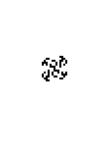
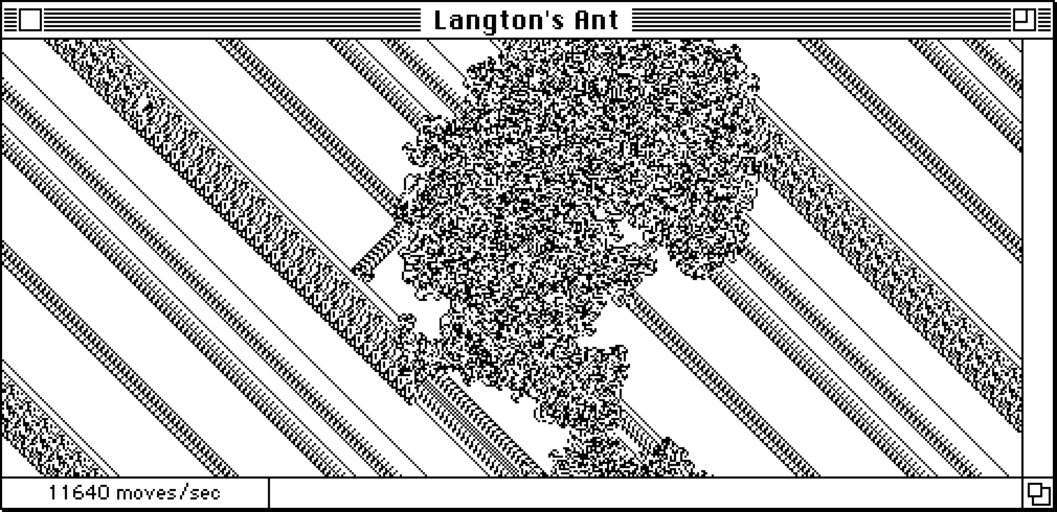
When the ant starts on a uniformly colored grid, it first produces simple symmetric patterns, then larger more chaotic patterns, and finally—after 10,000 or so moves—an emergent pattern: a regular highway that extends indefinitely (assuming the grid is unbounded):

The ant exhibits other behaviors depending on the starting conditions. For example, by cleverly constructing and interpreting the state of the grid, the ant can implement boolean circuits, and ultimately simulate an arbitrary Turing machine, making it capable of universal computation.^[PDF]

I first read about Langton’s ant when I was a teenager in the early ’90s. Since this was pre-Web, my access to computer information was limited to magazines and local library books, so I’m not sure where I discovered it. A few years later, in college, I implemented it as screensaver for BeOS. I remember being mesmerized by the ant zipping around the screen. It felt like watching something elemental.

Because of my interest in retrocomputing, and because Langton’s ant was invented in the mid-80s, I started to wonder how it would have performed on my family’s home computers of that era: a Commodore 64 and a Macintosh Plus. As a kid, I didn’t have the skills necessary to make a graphical Macintosh app in C, or to write a 6502 assembly program for the Commodore 64. I’ve learned a few things since then, so I thought it would be fun to create those programs now.

The rest of this article will examine some of the implementation details of Langton’s ant for an old-school Macintosh: Langtons-Ant-68k-Mac, and for the Commodore 64: LANGTON64. We’ll also take a look at a version that runs in a terminal emulator on a modern-day computer: langtons-termite.

Common Functionality

To implement Langton’s ant, we need to:

• Track the $(x,y)$ coordinates of the ant on the grid.
• Find the pixel corresponding to that location.
• Turn the ant right or left based on the pixel value.
• Invert the pixel color.
• Move to the next cell.

Each project uses a 1-bit bitmap to represent the grid. Finding the ant’s pixel requires us to find the correct byte in that bitmap, and the correct bit in that byte. Most of the platform-specific discussions in the following sections will relate to how the bitmap is structured in memory and how we can inspect and modify it. First, though, we’ll take a look at some of the higher level details that are common to all of the programs.

Life on a Torus

Watching the ant extend its highway on an unbounded grid gets boring quickly—and our bitmaps are very much bounded—so we actually want the grid to behave like the surface of a torus rather than a plane. On a torus, the ant can still move indefinitely in any direction, but it will eventually wrap around to its previous location.

Practically, this means that we need to warp the ant to the opposite side of the bitmap when it’s about to fall off the edge. With this behavior, the highway will eventually run into an old portion of the trail that interrupts the pattern. This causes the ant to reenter a chaotic state. If there are still unvisited cells, the highway will reemerge—often shooting off in a new direction. If allowed to run long enough, the ant will fill the entire bitmap with seemingly random noise, leaving the ant in a permanent state of chaos.

One wrinkle of mapping the grid to a torus is that the parity of the bitmap size affects the way the ant interacts with its trail. The programs described here will normally use an even width and height for the bitmap. However, the Macintosh app switches to an odd width and height if you hold down the shift key while resizing the window.

With odd dimensions, the ant seems to go “out of phase” when it wraps at a bitmap boundary. It will modify its old highways in a variety of ways, sometimes undoing them completely. Even-sized grids do not exhibit this behavior. This is probably related to the fact that the highway pattern is 104 steps long and shifts the ant 2 pixels horizontally and 2 pixels vertically every iteration.

Turning Left and Right

We need a way to turn the ant left or right. One way to implement this is to map the cardinal directions to sequential integers in a clockwise fashion:

North = 0
East  = 1
South = 2
West  = 3

A right turn is then equivalent to adding 1 to the current orientation modulo 4, and a left turn is equivalent to subtracting 1 from the current orientation modulo 4.

Because $x \bmod 2^n = x\space\&\space(2^n-1)$, and 4 is a power of 2, we can compute the mod operation using a bitwise AND:

turnRight orientation = (orientation + 1) & 0x3
turnLeft  orientation = (orientation - 1) & 0x3

This bitwise modulo trick will appear frequently in these projects.

Generating Random Dots

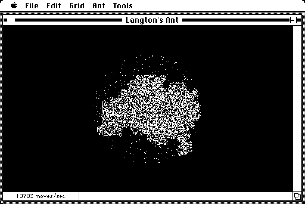
It’s conjectured that the ant—on an infinite grid—will always build a highway given any finite starting configuration. For my BeOS screensaver, I wanted to test that theory by adding random “dirt” within a circle around the ant’s starting position. The idea was to see how long it would take the ant to escape the circle of dots via its usual highway.

Initially, I used random polar coordinates to generate the dots. If the target circle has radius $r$, we generate one random number, $m$, in the range $[0, r)$ for the magnitude, and another random number, $\alpha$, in the range $[0, 2 \pi)$ for the angle. Then we convert those values to Cartesian coordinates using some trigonometry:

$$ \begin{aligned} x &= m \cdot \cos \alpha \newline y &= m \cdot \sin \alpha \end{aligned} $$

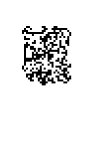
This works, but calling two trigonometric functions per point is expensive for our 1980s CPUs. Also, while there’s no wrong way to generate a random mess for the ant, this method does tend to clump points in the center of the circle (see Figure 1 below).

An alternative method is to generate random points within the square that encloses the circle, and toss out the points that fall outside the circle. This is similar to the Monte Carlo method for estimating the value of $\pi$:

If the circle has radius $r$, the enclosing square has width and height $2r$. So we generate two random values $x$, and $y$, in the range $[0, 2r)$. The generated point $(x, y)$ is now somewhere inside the square. If the distance from that point to the center of the square, $(r, r)$, is less than the radius of the circle, the point is good, otherwise, we need to discard it and try again. We can use the Pythagorean theorem to test the distance:

$$ (x-r)^2 + (y-r)^2 < r^2 $$

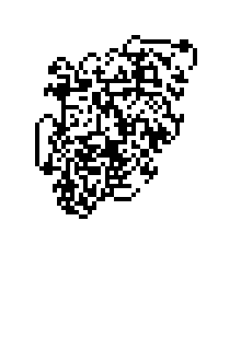
This method requires that we generate more random points than we use—to get $n$ points in the circle, we need to generate $4n/\pi$ dots on average—but it avoids trigonometric functions and produces a uniform distribution of points within the circle (see Figure 2). We’ll use this technique for the programs described here.

Turning Back Time

The behavior of Langton’s ant is reversible—we can rewind time, causing the ant to undo its previous efforts. Recall that the ant’s action is turn–invert–move. To reverse the ant:

• Flip the ant’s orientation so that it’s facing in the opposite direction (i.e. rotate it 180°).
• Move forward one cell (so that the ant returns to its position prior to its last action).

Then continue normally: turn–invert–move.

No matter how chaotic the mess on screen, reversing the ant will eventually return the grid to its starting configuration. It’s satisfying to watch. This reversibility also suggests its potential use as an encryption algorithm.

Classic Macintosh

My dad bought a Mac Plus in October 1987, when I was 11 years old. It had an 8MHz Motorola 68000 CPU, 1MiB of RAM, and a built-in monochrome display with a resolution of 512 × 342 pixels. He later maxed out the RAM at 4MiB, and added an external 40MiB hard drive that sat under the computer, raising it to a more ergonomic height.

I fell in love with the Mac immediately. Even though the display was only black and white, it made up for it by being high-resolution and beautiful. I used the Plus for school work, played Dark Castle, and created bitmap graphics with SuperPaint. My dad was a photojournalist and had access to laser printers at the local newspaper where he worked. I was fascinated with Adobe Illustrator and its ability to produce mathematically pure curves that looked pixelated on my screen, but gorgeous when laser-printed at 300dpi. I would send a floppy off with my dad and wait for the results.

I also used HyperCard a lot. I wanted to make my own Mac apps, but I didn’t have the C programming skills to make a “real” app. HyperCard was empowering. I made a HyperCard stack called TeleCanvas that could connect to another instance of TeleCanvas over a dial-up modem and transmit doodles back and forth on a shared canvas. I was only able to test it once or twice with a colleague of my dad’s. It worked! We played tic-tac-toe.

I still have that Mac Plus and it still works great. I used it to test this project, which I developed on a modern Linux system with the Retro68 project. I avoided using any modern C conventions so that the code can still be compiled with an era-appropriate compiler (THINK C) running natively on a 68k-based Macintosh. The modern compiler produces a binary that is twice as fast—and twice as big—as the classic compiler. You can read more about that, how to build it, and how to run it in an emulator on the project page.

In addition to the general capabilities already described, the Mac app provides drawing tools—a pencil and an eraser—and an option to use random shapes as a starting configuration. It also supports copy and paste, allowing you to paste in any bitmap image as a starting configuration.

App Setup

This app displays Langton’s ant in a single resizable window. An offscreen bitmap is updated by the ant and periodically copied to the screen.

Mac apps are event-driven—they run in an infinite loop, processing events from the system and the user. Events are things like mouseDown, keyDown, and updateEvt (the system indicating we need to redraw the window).

We want the ant to move whenever we’re not processing another event. If there are no pending events—a virtual “idle event”—we run the ant for a short time and copy the result to the screen before checking for another event. Running in brief bursts allows the user interface to remain responsive.

The HandleIdleEvent() function tries to settle on the number of moves per idle event that produces around 40 screen updates per second. 60 updates per second would better match the screen refresh rate, but the Mac Plus performs better with a slower frame rate. To run the ant, HandleIdleEvent() calls the RunAnt() function—which we will examine later.

The Mac’s imaging library is called QuickDraw. It provides functions for drawing shapes, images, and text. One of the main data structures used by QuickDraw is a GrafPort—a pointer to which is a GrafPtr. This is a graphics context that points to a bitmap, and tracks state that affects drawing, like clipping regions, patterns, and pen sizes.

The current graphics port is a global variable implicitly referenced by most QuickDraw functions. Normally, you call SetPort() with the appropriate GrafPort before issuing QuickDraw commands to make sure you’re affecting the bits that you intend to affect. We’ll set up a GrafPort for the offscreen bitmap so that we can render into it with QuickDraw functions—we’ll use that capability to add random shapes to the grid.

To implement Langton’s ant, we could use QuickDraw functions like GetPixel(), MoveTo(), and LineTo() to query the pixels of the bitmap and alter them, but this would be slow. In this case, we want to modify the bits of the bitmap directly. In order to do that, we need to take a closer look at QuickDraw’s BitMap structure.

QuickDraw BitMaps

QuickDraw’s BitMap structure looks like this:

struct BitMap {
    char  *baseAddr;
    short rowBytes;
    Rect  bounds;
};

The bytes of a BitMap are a single contiguous allocation pointed to by baseAddr. Each byte represents a horizontal sequence of 8 pixels—1 pixel for each bit in the byte. A bit value of 0 produces a white pixel, and a bit value of 1 produces a black pixel.

The rowBytes field indicates the number of bytes per row of the image—in other words, how many bytes are displayed horizontally before advancing vertically to the next row of pixels. rowBytes provides the information needed to turn the 1-dimensional array of bytes into a 2-dimensional image.

To inspect and alter the pixel at $(x,y)$, we have to find the byte that contains it. Since we want the $y$th row, and there are rowBytes bytes per row, we find the byte’s row by multiplying:

row = y * bitmap->rowBytes

Since there are 8 pixels per byte, we find the column of the byte by dividing:

col = x / 8

The correct byte is then at baseAddr[row + col].

Once we have the appropriate byte, we need to generate a bit mask to isolate the correct bit. To do that, we start with the mask 0x80—binary value 0b1000_0000— and shift it to the right by the remainder of $x$ divided by 8. This catches the overflow from the column calculation above, and scoots it into the byte:

mask = 0x80 >> (x % 8)

Putting it all together, we can find the value of a pixel like so:

char MyGetPixel(BitMap *bitmap, short x, short y) {
    // find the row containing the target byte
    short row = y * bitmap->rowBytes;
    // find the column of the target byte
    short col = x / 8;
    // mask for the target bit
    Byte  mask = 0x80 >> (x % 8);

    return bitmap->baseAddr[row + col] & mask;
}

A function to invert the pixel is nearly identical, but uses the exclusive or operator to toggle the bit:

void InvertPixel(BitMap *bitmap, short x, short y) {
    // find the row containing the target byte
    short row = y * bitmap->rowBytes;
    // find the column of the target byte
    short col = x / 8;
    // mask for the target bit
    Byte  mask = 0x80 >> (x % 8);

    bitmap->baseAddr[row + col] ^= mask;
}

Marching Ants

Now we’ll take a look at the core functionality of the app. Here is the main data structure, Grid, and its associated enums:

typedef enum {
    StartEmpty,
    StartWithRandomDots,
    StartWithShapes
} StartState;

typedef enum { North, East, South, West} Cardinal;

typedef struct {
    WindowPtr  window;
    BitMap     bits;
    short      width, height;
    // position of ant
    short      x, y;
    Cardinal   orientation;
    // extent of ant movement for dirty rect
    short      minx, maxx, miny, maxy;
    // status variables
    Boolean    paused;
    Boolean    moveBackward;
    StartState initialState;
    short      mode;
    // for offscreen QuickDraw rendering
    GrafPtr    port;
    // optimizations
    int        currentRow;
    int        maxRow;
} Grid, *GridPtr;

Grid manages bits as an offscreen bitmap—this is where the ant will work. width and height cache the size of the image for quick access.

The window member points to the window with which the Grid is associated. mode is a QuickDraw value that determines whether or not we are inverting the grid (set to srcCopy for the default rendering and srcNotCopy for inverted rendering). The port member allows us to render into bits with QuickDraw commands.

x and y track the ant’s location, and currentRow tracks the ant’s row within the bitmap. Since the ant only moves 1 pixel at a time, we can add bits->rowBytes to currentRow to move down 1 pixel (or subtract it to move up 1 pixel). This eliminates the need for a more expensive multiplication like we saw in MyGetPixel() above. maxRow serves a similar purpose and is cached so we can quickly warp from the 0th row to the last row of the bitmap.

As the ant moves, we track its range with minx, maxx, miny, and maxy. These variables determine the dirty rectangle—the area of the image that’s actually changed. When we update the screen, we copy only the bits in the dirty rectangle. The smaller the rectangle copied to the screen, the faster the update.

When a Grid is created, and when the ant is reset, CenterAnt() is called to initialize the variables that track the ant:

void CenterAnt(GridPtr grid) {
    grid->x = grid->width / 2;
    grid->y = grid->height / 2;
    grid->currentRow = grid->y * grid->bits.rowBytes;
    grid->orientation = grid->moveBackward ? East : West;

    grid->minx = grid->maxx = grid->x;
    grid->miny = grid->maxy = grid->y;
}

As mentioned earlier, RunAnt() is called whenever we have an “idle” event. RunAnt() loops numSteps times, repeatedly executing the ant’s turn–invert–move action, then flushes the dirty rectangle to get the modified pixels on screen (more on that later).

RunAnt() merges the MyGetPixel() and InvertPixel() functions shown earlier. As optimizations, it uses a bit shift to substitute for division by 8, and applies the bitwise modulo technique discussed in the Turning Left and Right section:

void RunAnt(GridPtr grid, short numSteps) {
    while (numSteps--) {
        // relevant byte is at (row + x / 8)
        int  ix = grid->currentRow + (grid->x >> 3);
        // relevant bit is (0b1000_0000 >> x % 8)
        Byte mask = 0x80 >> (grid->x & 0x7);
        // was the image bit on or off?
        Byte pixel = grid->bits.baseAddr[ix] & mask;

        // invert the image bit
        grid->bits.baseAddr[ix] ^= mask;

        // turn left if pixel was on, otherwise turn right
        grid->orientation += pixel ? -1 : 1;
        grid->orientation &= 0x3;

        // move forward one cell
        Step(grid);
    }

    FlushDirtyRect(grid);
}

RunAnt() also calls Step() to actually move the ant:

void Step(GridPtr grid) {
    switch (grid->orientation) {
    case North: DecrY(grid); break;
    case East: IncrX(grid); break;
    case South: IncrY(grid); break;
    case West: DecrX(grid); break;
    }
}

Step() hands off all the work to helper functions, like DecrY() below:

void DecrY(GridPtr grid) {
    grid->y--;
    grid->currentRow -= grid->bits.rowBytes;

    if (grid->y < 0) {
        // warp to bottom
        grid->y = grid->height - 1;
        grid->currentRow = grid->maxRow;

        FlushDirtyRect(grid);
    } else if (grid->y < grid->miny) {
        grid->miny = grid->y;
    }
}

DecrY() decrements grid->y and grid->currentRow. If grid->y is negative, the ant is warped to the bottom of the bitmap. The dirty rectangle is flushed when warping because it would otherwise span the entire height of the image, making it much bigger than necessary. If no warp occurs, grid->miny is updated to track the top of the dirty rectangle.

IncrY(), DecrX(), and IncrX() all work similarly.

Finally, we need to take a look at FlushDirtyRect(), which makes the offscreen bitmap visible on screen:

void FlushDirtyRect(GridPtr grid) {
    BitMap *gridBits = &grid->bits;
    BitMap *windowBits = &grid->window->portBits;
    Rect   rect;

    rect.top    = grid->miny;
    rect.left   = grid->minx;
    rect.bottom = grid->maxy + 1;
    rect.right  = grid->maxx + 1;

    CopyBits(gridBits, windowBits, &rect, &rect, grid->mode, NULL);

    grid->minx = grid->maxx = grid->x;
    grid->miny = grid->maxy = grid->y;
}

This function converts the range tracking variables into a proper QuickDraw Rect and copies the bits in that rectangle from the offscreen bitmap into the window’s bitmap. It passes grid->mode to CopyBits() to invert the image if necessary. Then it resets the range tracking variables for the next update.

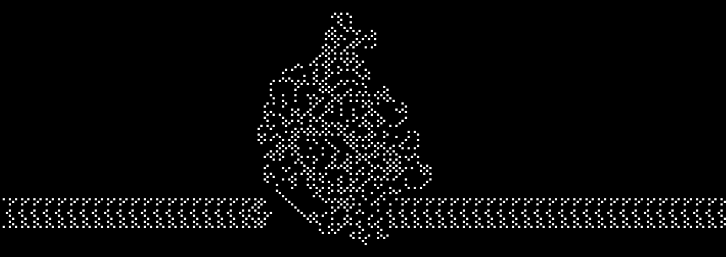
Ant-Aliasing

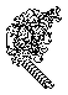
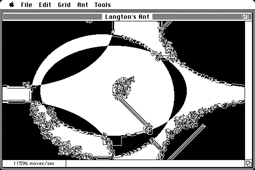
In addition to adding random dots to the grid, the Mac app allows you to add random shapes. Langton’s ant has a tendency to follow edges, displacing pixels, but preserving the essence of the shapes it encounters—at least initially:

We can create elaborate patterns using only three ovals rendered with PenMode(patXor). Because of the patXor mode, each oval inverts the area of the previous ovals that it intersects. To respect the coordinate rules of the torus-grid, ovals that get clipped by the edges of the bitmap must be offset and re-rendered so that they wrap around the torus. In the worst case scenario, an oval must be drawn four times to reach every corner of the grid:

void AddShapes(GridPtr grid, short numShapes) {
    Rect    shapeRect;
    Boolean wrapHorizontal, wrapVertical;
    short   minWidth = grid->width / 2;
    short   minHeight = grid->height / 2;

    PenMode(patXor);

    while (numShapes--) {
        // generate x and y anywhere inside the grid
        short x = URandom() % grid->width;
        short y = URandom() % grid->height;
        // generate width in range [minWidth, minWidth * 2)
        short width = minWidth + URandom() % minWidth;
        // generate height in range [minHeight, minHeight * 2)
        short height = minHeight + URandom() % minHeight;

        SetRect(&shapeRect, x, y, x + width, y + height);
        PaintOval(&shapeRect);

        wrapHorizontal = shapeRect.right > grid->width;
        wrapVertical = shapeRect.bottom > grid->height;

        if (wrapHorizontal) {
            MoveRectTo(&shapeRect, x - grid->width, y);
            PaintOval(&shapeRect);
        }

        if (wrapVertical) {
            MoveRectTo(&shapeRect, x, y - grid->height);
            PaintOval(&shapeRect);
        }

        if (wrapHorizontal && wrapVertical) {
            MoveRectTo(&shapeRect, x - grid->width, y - grid->height);
            PaintOval(&shapeRect);
        }
    }

    PenMode(patCopy);
}

Wrap-Up

This section has primarily focused on how to work with QuickDraw’s BitMap data structure. I haven’t elaborated on other details of the app, like how the user interface is set up and managed. This is a big topic—see the references below—and beyond the scope of this article.

However, as a starting point, in LangtonsAnt.c, you’ll find code to create the application window, handle mouse events, and deal with menu selections. The most interesting function is probably TrackDrawingTool(), which handles the pencil and eraser tools. You’ll also find EventLoop(), which runs the whole show.

If you’re interested in doing your own retro-Macintosh programming, I recommend the Inside Macintosh series of books produced by Apple. There are many volumes, but this is a good place to start:

• Overview (PDF)
• Macintosh Toolbox Essentials (PDF)
• Imaging with QuickDraw (PDF)

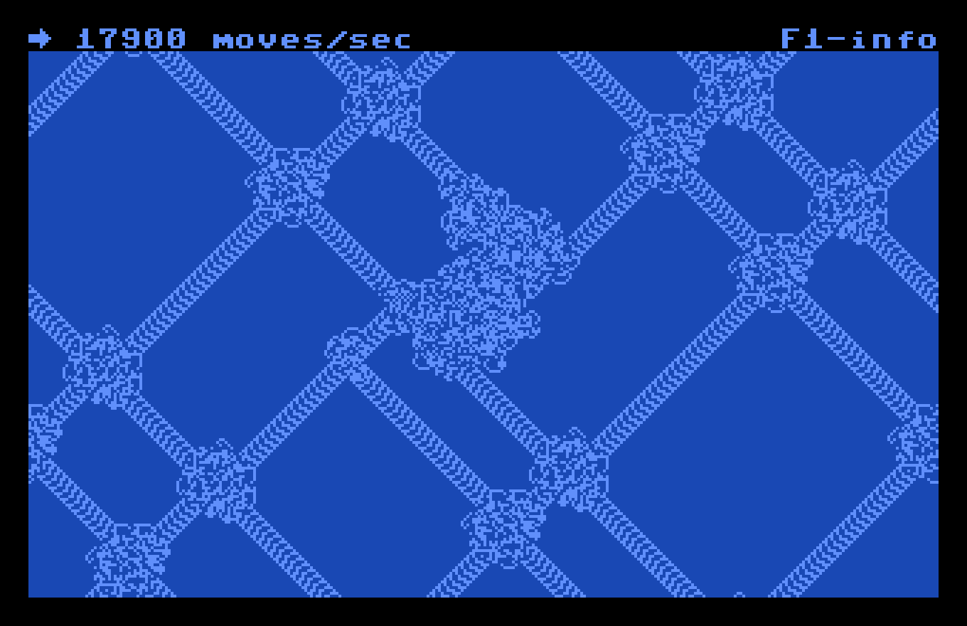
Commodore 64

The Commodore 64 (C64) was our family’s second home computer (the first was a Timex Sinclair 1000). As a kid, I never got beyond programming with BASIC on the C64. I remember being interested in assembly language, but we didn’t have an assembler, and I didn’t pursue it. By the time my interest in computers truly blossomed, we had the Mac Plus, and I was enamored with the idea of high-resolution graphical interfaces.

In addition to its 6502 processor—technically a 6510—the C64 has custom chips for graphics (the VIC-II), and sound (the SID). The VIC-II supports multiple character and bitmap modes (320 × 200 pixels in high-res), 16 colors, and 8 sprites. Over the last 40 years, demoscene artists have pushed the C64 to its absolute limits. There are many amazing demos that defy the apparent limitations of the hardware.

The C64 has 64KiB of unconstrained mutable state (i.e. RAM), just like it says on the tin. The memory map is fairly complex, with certain regions designated for screen characters, colors, sprites, and so on. Some memory locations are mapped to registers for the VIC-II and the SID, which is how you configure them programmatically. Because the VIC-II can only see a bank of 16KiB of RAM at a time, locations for graphical content depend on how the VIC-II is configured. Since there’s nothing to stop you from changing any value in memory at any time, care is warranted.

Programming the C64 in assembly is fun—especially if you can do it from the comfort of a modern system. I found instruction level optimization particularly satisfying because there are no intervening layers of abstraction between you and the machine. You can add up the cycles in your loops with pen and paper, leaving no doubt when you’ve improved performance. I highly recommend it if you’ve never tried it before.

I initially hoped that LANGTON64, the C64 version of Langton’s ant, would achieve at least half the number of moves per second as the Mac Plus, which can do around 10,000. The C64 ended up trouncing the Plus, getting around 18,000 moves per second. This is despite the Plus operating at 8MHz and the C64 operating at 1MHz.

The Commodore program does have a few advantages. First, I spent a lot of time hand-optimizing the assembly code. Second, this program modifies screen memory directly, so it doesn’t have to copy image data around or track a dirty rectangle. Still, I was impressed with the performance. Someone who knows 68000 assembly could undoubtedly squeeze more speed out of the Mac.

I developed LANGTON64 on a Linux system with the ACME Cross-Assembler, and tested it with the VICE emulator. I also tested it on an Ultimate 64, a modern FPGA-based C64. You can find the code and build instructions on the project page.

6502 Basics

A tutorial for 6502 assembly is beyond the scope of this article, but here are a few basics.

The 6502 processor was used in the C64, Apple II, BBC Micro, original Nintendo, and many other machines. It is an 8-bit processor, meaning it can only operate on a single byte at a time. It does, however, use 16-bit addressing, allowing it to access 64KiB of memory. The 6502 is little-endian, so the first byte of an address is the low byte.

It has three registers: A, X, and Y. The A register—the accumulator—is used by the mathematical and logical instructions. X and Y are often used as indices in different addressing modes. Many instructions work with one of these registers, but some can also operate directly on memory.

There are instructions for adding, subtracting, performing bitwise operations, loading registers, storing registers, comparing, and branching. Notably missing are any instructions for multiplying and dividing.

The 6502 has a large number of addressing modes. An addressing mode is a way of specifying the source of an instruction’s operand. Here’s a subset commonly used in LANGTON64, with the LDA (LoaD Accumulator) instruction serving as an example:

• Immediate: A constant value is provided with the instruction. LDA #100
• Absolute: A memory location is directly specified. LDA $d020
• Absolute Indexed: The X or Y register is added to an absolute address to determine the memory location to use. This is often used in a loop, where the value of the X or Y register changes on each iteration, allowing you to walk through memory. LDA $d020,x
• Zero Page: An absolute location in the first 256 bytes of memory. The zero page can be accessed faster than other memory locations, so it’s a good place to stash frequently used variables. LDA $02
• Indirect Indexed: A zero page location used as a pointer to another memory location, to which the Y register is then added. We’ll use this mode to manage a bitmap pointer. LDA ($02),y

Since optimizing assembly comes down to counting CPU cycles per instruction, it’s worth noting that branching instructions like BEQ (Branch if EQual to zero), and BNE (Branch if Not Equal to zero), take 3 CPU cycles when the branch is taken, and only 2 cycles if the branch is not taken. If you know the odds that a branch will be taken, you can optimize your code by choosing the branch case that will occur less frequently.

Program Setup

The starting point for LANGTON64 is langton.a. The code here initializes variables, copies character images from ROM to RAM (so that they can be customized), sets up screen colors, and clears the bitmap memory region. It switches the machine from character mode to bitmap mode, then executes mainLoop:

mainLoop:
        lda flags
        bne @handleFlags
@runAnt jsr runAnt
        +add16_byte moves, MOVES_PER_LOOP
        jmp mainLoop
@handleFlags
        and #KEYBOARD_FLAG
        beq +
        jsr checkKeyboard
+       lda flags
        and #MOVES_STALE_FLAG
        beq +
        jsr updateMovesPerSecond
+       lda flags
        and #(PAUSE_FLAG | INFO_FLAG)
        beq @runAnt
        bne mainLoop

mainLoop loads the flags zero page variable, and if it’s zero, jumps to the runAnt subroutine to run the ant, otherwise it handles any flags that are set. The flags variable can indicate any combination of the following states:

• KEYBOARD_FLAG The keyboard should be checked for user input.
• MOVES_STALE_FLAG The “moves/second” field in the status line should be updated.
• PAUSE_FLAG The ant is paused.
• INFO_FLAG The program is displaying the “Info” screen.

KEYBOARD_FLAG and MOVES_STALE_FLAG are set by an interrupt handler, irq_tick, which is triggered by the system every tick (1/60 of a second). KEYBOARD_FLAG is set every tick, and MOVES_STALE_FLAG is set every 60 ticks. PAUSE_FLAG and INFO_FLAG are set in response to keyboard input from the user.

High-Resolution Bit Map Mode

The C64 has a number of different character and bitmap display modes. However, it always has a character-centric view of the world, even when it’s in a bitmap mode.

In standard character mode, the screen is composed of 1000 character codes arranged in a 40 × 25 grid. You alter the image on screen by changing one of the character codes in the grid, or by modifying the character image for a given character code. Each character image is an 8 × 8 grid of pixels—8 bytes arranged in a vertical stack. Only 256 characters are active at a time, so it’s not possible to directly control every pixel on screen.

In standard high-resolution bitmap mode, each pixel is directly modifiable, but the bytes are still arranged as if they are in a grid of characters. Instead of a grid of 40 × 25 character codes, it’s a grid of 40 × 25 character images. This makes working with the pixels in the bitmap a bit awkward. The Commodore 64 Programmer’s Reference Guide provides this formula for finding a pixel (starting on page 125):

byteForPixel (x, y) = BITMAP_BASE + (y / 8) * 320 + (y % 8)
                                  + (x / 8) * 8

maskForPixel (x, _) = 0x80 >> x % 8

This is a lot of math for the 6502, especially since there are no CPU instructions for multiplication and division. We can work around this by using lookup tables, demonstrated here by the drawPixel routine. This routine is used when drawing random dots. The pixel’s $x$ coordinate is passed in the X register and the $y$ coordinate is passed in the Y register:

drawPixel:
        ;; --- load y component of byte's address into bitmap_ptr
        lda @row_lo,y
        sta bitmap_ptr
        lda @row_hi,y
        sta bitmap_ptr+1
        ;; --- compute x component of byte's address
        txa                ; A <- x
        and #$f8           ; A <- (x DIV 8) * 8
        tay                ; Y <- (x DIV 8) * 8
        ;; --- draw the pixel
        lda (bitmap_ptr),y
        ora @masks,x       ; turn pixel on
        sta (bitmap_ptr),y
        rts
@masks  !for i, 0, 255 { !byte $80 >> i % 8 }
@row_lo !for y, 0, 199 { !byte < BITMAP_BASE + y DIV 8 * 320 + y % 8 }
@row_hi !for y, 0, 199 { !byte > BITMAP_BASE + y DIV 8 * 320 + y % 8 }

As written, this routine only works with an 8-bit $x$ coordinate, so it can’t cover the entire width of the screen (320 pixels). This is sufficient for drawing random dots in the middle of the screen, but if we wanted to use the same technique for rendering Langton’s ant, we’d have to adjust it to accept a 16-bit $x$ coordinate.

Character is Destiny

The lookup table technique works well for drawing an arbitrary pixel, but it may not be the best fit for managing the ant. To test and alter a pixel anywhere on screen, we would need to use a 16-bit $x$ coordinate to track the ant. Every move would require a 16-bit addition to combine the $x$ and $y$ components of the byte’s location. Often this addition would be redundant because the ant didn’t actually move into a new byte.

We can do better if we take advantage of our knowledge of the bitmap structure, and the fact that the ant never moves more than one pixel in any given direction (ignoring torus warping for the moment). In fact, we don’t need a lookup table, and we don’t need to explicitly track the ant’s $(x,y)$ coordinates at all.

An alternative idea is to treat each 8 × 8 character region as a mini-bitmap that can contain the ant. As long as the ant stays within the same character region, it can be moved with just a couple of instructions. There is some extra bookkeeping when the ant transitions to a neighboring character region, but this is easy to detect, and happens relatively infrequently.

In order to efficiently track the ant, we will use the following variables, all stored in the zero page:

• ant_char_ptr A pointer to the first byte in the ant’s current character region.
• ant_char_y An offset from ant_char_ptr, in the range $[0,7]$. It indicates the byte within the character that contains the ant.
• ant_mask A byte with a single on-bit that identifies the ant’s pixel within the byte.
• ant_row The row of the ant’s character region.
• ant_col The column of the ant’s character region.

During the runAnt routine, ant_char_y will be loaded into the Y register. The ant’s byte can then be found using indirect indexing: (ant_char_ptr),y. The row and column of the ant’s character determine how to adjust ant_char_ptr when the ant moves into a neighboring region. These variables, along with the ant’s orientation, are initialized in the resetAnt routine.

The setup is illustrated in Figure 3 below. In this example, ant_char_ptr is set to memory location $30e0 (within the character region in column 20 and row 13). The Y register has been loaded with the value of ant_char_y, which is 4, so, (ant_char_ptr),y points to the byte at $30e4

The on-bit in ant_mask isolates a single bit in a byte. If we AND the mask with the byte at $30e4, we get the current value under the ant. If we instead use EOR (Exclusive OR), we toggle the color of the pixel under the ant.

We can move the ant 1 pixel east by rotating ant_mask 1 bit to the right using the LSR (Logical Shift Right) instruction, or 1 pixel west by rotating ant_mask 1 bit to the left using the ASL (Arithmetic Shift Left) instruction. In either case, if the carry bit is set after the rotation, we know that the ant has left the current character region. To move into a new region, we need to increment or decrement ant_col, and make the corresponding adjustments to ant_mask and ant_char_ptr. That happens in separate subroutines I’ll describe later.

Similarly, to move the ant 1 pixel north, we decrement the Y register using the DEY (DEcrement Y) instruction. To move 1 pixel south, we increment Y using the INY (INcrement Y) instruction. If the value of Y is out of the range $[0,7]$, the ant has moved into a new character region, and we will need to increment or decrement ant_row and adjust ant_char_ptr (again, this is handled by separate subroutines).

This is all put together in the runAnt routine:

runAnt:
        ldx #MOVES_PER_LOOP ; assumes no other use of X during loop
        ldy ant_char_y      ; Y <- ant_char_y
        ;; --- invert the pixel ---
@loop   lda (ant_char_ptr),y
        eor ant_mask        ; invert the pixel
        sta (ant_char_ptr),y
        ;; --- turn the ant ---
        and ant_mask        ; see if the pixel was on or off
        beq @left           ; if 0, pixel was on before `eor' above
@right  inc ant_orientation
        lda ant_orientation ; A <- ant_orientation
        and #3              ; A <- ant_orientation % 4
        beq @north          ; A == 0
        cmp #2
        bcc @east           ; A == 1
        beq @south          ; A == 2
        bcs @west           ; A == 3
@left   dec ant_orientation
        lda ant_orientation ; A <- ant_orientation
        and #3              ; A <- ant_orientation % 4
        beq @north          ; A == 0
        cmp #2
        bcc @east           ; A == 1
        beq @south          ; A == 2
        ;; --- move forward one cell ---
@west   asl ant_mask
        bcs +               ; will only branch 1/8 of time
        +next @loop         ; still within current char
+       jsr decrementCol    ; carry set: move west 1 char
        +next @loop
@east   lsr ant_mask
        bcs +               ; will only branch 1/8 of time
        +next @loop         ; still within current char
+       jsr incrementCol    ; carry set: move east 1 char
        +next @loop
@north  dey
        bmi +               ; will only branch 1/8 of time
        +next @loop         ; still within current char
+       jsr decrementRow    ; Y < 0: move north 1 char
        +next @loop
@south  cpy #7              ; Y == 7 ?
        beq +               ; will only branch 1/8 of time
        iny                 ; still within current char
        +next @loop
+       jsr incrementRow    ; Y == 7: move south 1 char
        +next @loop

runAnt loops to amortize the expense of calling it as a subroutine from mainLoop. It utilizes a macro, next, to manage the loop—this makes it easy to inline the same instructions in multiple places. When the loop ends, next stores the value of the Y register in ant_char_y before returning:

!macro next @a {
        dex
        bne @a
        sty ant_char_y
        rts
}

Now we need to examine the subroutines that move the ant into a new character region. Here’s the code for incrementCol, which advances the ant one character to the east:

incrementCol:
        ror ant_mask  ; rotate in carry bit (now %1000_0000)
        lda ant_col
        cmp #MAX_COL  ; ant_col == MAX_COL ?
        beq @warp     ; warp if we're in the max column
        inc ant_col
        +add16_byte ant_char_ptr, COL_DELTA
        rts
@warp   lda #MIN_COL  ; jump to leftmost column
        sta ant_col
        +sub16 ant_char_ptr, SCREEN_WIDTH
        rts

The carry bit is rotated into ant_mask, putting it on the left side of the byte. If ant_col is the rightmost column, ant_col and ant_char_ptr are warped to the left side of the bitmap. Otherwise, ant_col and ant_char_ptr are shifted one character region to the right. The code for decrementCol is analogous.

The incrementRow and decrementRow routines are also similar. They don’t need to touch ant_mask, but they do have to modify the Y register:

incrementRow:
        ldy #0        ; Y <- first byte in char
        lda ant_row
        cmp #MAX_ROW  ; ant_row == MAX_ROW ?
        beq @warp     ; warp if we're in the max row
        inc ant_row
        +add16 ant_char_ptr, ROW_DELTA
        rts
@warp   lda #MIN_ROW  ; jump to top row
        sta ant_row
        +sub16 ant_char_ptr, SCREEN_HEIGHT
        rts

On average, we only need to jump to one of these subroutines once for every 8 ant movements (12.5% of the time). If you consider the ant_mask byte, for example, 7 out of 8 rotations will not modify the carry bit—meaning there’s no need to change ant_col. The same logic applies to incrementing and decrementing Y with respect to ant_row.

Wrap-Up

As in the previous section on the Mac, I focused on the details related to the C64’s bitmap mode without expounding much on the rest of the program. If you want to dig in, the entry point for the program is in langton.a. User input is managed by routines in input.a. Routines for updating the status line are in status.a. Random dot generation is handled by dots.a > randomDots.

If you want to program the C64, you’ll probably want a copy of the Commodore 64 Programmer’s Reference Guide. I was able to find a physical copy on eBay. There are also loads of resources on the web—here are a few that I found useful:

• Codebase 64
• C64 Wiki
• Dustlayer
• Easy 6502

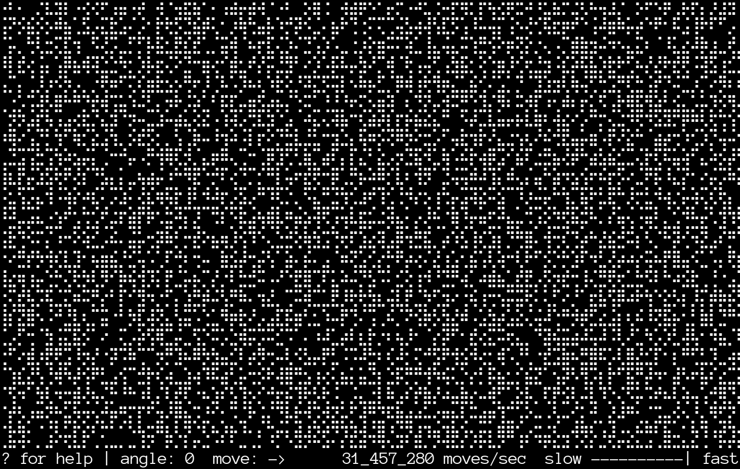
Terminal Emulator

I initially wanted to run Langton’s ant in a terminal emulator because I wanted to try using Braille Unicode characters to represent pixels (as many preexisting projects have done). The result was langtons-termite, which I wrote in Rust. I used Termion to interact with the terminal.

Compared to the C64 and Mac Plus, a modern computer has seemingly infinite resources. While the Plus can get up to 10,000 moves per second, and the C64 can do 18,000 moves per second, my modern—6 year old—desktop can easily do 10s of millions of moves per second. The Mac Plus and C64 programs always go all out, running Langton’s ant as fast as they can. Because of the tremendous speed of a modern machine, langtons-termite allows you to control the rate at which the ant moves, from 30 moves per second to millions of moves per second.

This is accomplished by updating the on-screen text at 30 frames per second, and varying the number of moves per frame using powers of 4. The lowest number of moves per frame is $4^0$ (1) and the highest is $4^{10}$ (1,048,576). At the fastest setting, the screen is more or less instantly filled with noise.

Braille Dots as Bits

As mentioned above, langtons-termite uses Braille Unicode characters to represent pixels on screen. Braille symbols are composed of 2 columns of 4 dots that are either on or off—a physical Braille symbol would have a raised bump for every “on” dot. Because there are 8 total dots, we can represent each Braille glyph with a single byte.

The dots in Braille are numbered 1 to 8, and can be mapped to bit positions within a byte as shown in Figure 4 below. The irregular dot pattern is due to the fact that Braille originally used only 6 dots. Dots 7 and 8 were appended to the bottom when they were added later.

This dot-to-bit mapping allows us to convert a Braille byte into the correct Unicode character by adding it to the base Braille character, which is at 0x2800:

fn byte_to_braille(byte: u8) -> char {
    // 0x2800 is the first Braille Unicode character
    char::from_u32(0x2800 + byte as u32).unwrap()
}

Each Braille byte is a miniature 2 × 4 bitmap, and the overall bitmap representation is a two-dimensional array of these bytes. This array is sized to fit within the terminal window, so if $w$ is the terminal width and $h$ is the terminal height, the array has dimensions $w \times h$, and represents a bitmap with dimensions $2w \times 4h$.

Like on the Mac and the C64, to inspect and modify a pixel in the bitmap, we must find the right byte and isolate the right bit. Because each glyph is 4 dots high, the row index of the byte is the pixel’s $y$ value divided by 4. Likewise, because the glyphs are 2 dots wide, the column index of the byte is the pixel’s $x$ value divided by 2.

In order to inspect and toggle the correct bit within the Braille byte, we need the matching bit mask. For each dot position in the Braille pattern, the desired mask is 1 << (dot - 1). This generates the lookup table below:

/// Braille dot-to-bit mapping
static BRAILLE_BITS: [[u8; 2]; 4] = [[0x01, 0x08],
                                     [0x02, 0x10],
                                     [0x04, 0x20],
                                     [0x40, 0x80]];

To find the correct mask within the lookup table, we need to find the appropriate row and column indices. This is similar to how we found the byte, but instead of dividing, we need to use the modulo operator. Since each glyph is 4 dots high, the row index of the bit mask is the pixel’s $y$ value modulo 4. Likewise, since the glyphs are 2 dots wide, the column index of the bit mask is the pixel’s $x$ value modulo 2.

Terminal Velocity

Putting this all together, here is the primary method for running the ant. In this code, self.x and self.y represent the pixel location of the ant:

pub fn move_termite(&mut self) -> (usize, usize) {
    let (char_x, char_y) = (self.x / 2, self.y / 4);
    let (bit_x,  bit_y)  = (self.x % 2, self.y % 4);

    let byte = &mut self.braille_bytes[char_y][char_x];
    let mask = BRAILLE_BITS[bit_y][bit_x];
    let pixel = *byte & mask;

    // turn
    self.orientation = match pixel {
        0 => self.orientation.right(),
        _ => self.orientation.left(),
    };

    // toggle pixel
    *byte ^= mask;

    // move forward one cell
    self.step();

    // return the affected char coordinates
    (char_x, char_y)
}

The returned character coordinates are used by the calling method, next_frame(), to keep track of the dirty characters for each frame. The program can then make sure that it only writes each changed character to the terminal once per frame: display_dirty_characters().

The step method moves the ant forward one cell based on its orientation. It’s not as simple as it could be because langtons-termite allows you to rotate the grid 45°. When rotated, the highways run horizontally and vertically.

fn step_north(&mut self) {
    // avoid potential underflow by adding height
    self.y += self.height - 1;
    self.y %= self.height;
}

fn step_south(&mut self) {
    self.y += 1;
    self.y %= self.height;
}

fn step_east(&mut self) {
    self.x += 1;
    self.x %= self.width;
}

fn step_west(&mut self) {
    // avoid potential underflow by adding width
    self.x += self.width - 1;
    self.x %= self.width;
}

fn step(&mut self) {
    match self.orientation {
        N => self.step_north(),
        S => self.step_south(),
        E => self.step_east(),
        W => self.step_west()
    }

    if self.rotated {
        //    N        N | E
        //  W-+-E  =>  --+--
        //    S        W | S
        match self.orientation {
            N => self.step_west(),
            S => self.step_east(),
            E => self.step_north(),
            W => self.step_south()
        }
    }
}

Final Thoughts

Langton’s ant lives by simple rules—implementing it is a suitable challenge for a budding programmer. Even so, the task has some depth and nuance.

This article focused on how to work with a single pixel in an image. If you are an experienced programmer, it may seem straightforward, but there are many details you need to understand to find a pixel’s corresponding byte and bit. And as we have seen, each platform presents its own idiosyncrasies.

I’ve worked on this project, off and on, for a long time. Whenever I’ve examined the code after time away, I find something that could be improved. In normal circumstances, you likely can’t spend so much time navel-gazing, but it can be enlightening to continue experimenting with the same small programs.

Langton’s ant doesn’t require much in the way of computing resources. Maybe you could try bringing it to life in some weird or unexpected place?